OTL Circuit Function#
import numpy as np
import matplotlib.pyplot as plt
import uqtestfuns as uqtf
The OTL circuit test function is a six-dimensional scalar-valued function. The function has been used as a test function in metamodeling exercises [BAS07] and sensitivity analysis [Moo10]. In [Moo10], a 20-dimensional variant was used for sensitivity analysis by introducing 14 additional inert input variables.
Test function instance#
To create a default instance of the OTL circuit test function:
my_testfun = uqtf.OTLCircuit()
Check if it has been correctly instantiated:
print(my_testfun)
Function ID      : OTLCircuit
Input Dimension  : 6 (fixed)
Output Dimension : 1
Parameterized    : False
Description      : Output transformerless (OTL) circuit model from Ben-Ari and Steinberg (2007)
Applications     : metamodeling, sensitivity
Description#
The OTL circuit function computes the mid-point voltage of an output transformerless (OTL) push-pull circuit using the following analytical formula:
where \(\boldsymbol{x} = \{ R_{b1}, R_{b2}, R_f, R_{c1}, R_{c2}, \beta \}\) is the six-dimensional vector of input variables further defined below.
Probabilistic input#
Two probabilistic input model specifications for the OTL circuit function are available as shown in the table below.
The default selection, based on [BAS07], contains six input variables given as independent uniform random variables with specified ranges shown in the table below.
Function ID     : OTLCircuit
Input ID        : BenAri2007
Input Dimension : 6
Description     : Probabilistic input model for the OTL Circuit function
                  from Ben-Ari and Steinberg (2007).
Marginals       :

 No.    Name    Distribution    Parameters       Description
-----  ------  --------------  ------------  --------------------
  1     Rb1       uniform      [ 50. 150.]   Resistance b1 [kOhm]
  2     Rb2       uniform       [25. 70.]    Resistance b2 [kOhm]
  3      Rf       uniform       [0.5 3. ]    Resistance f [kOhm]
  4     Rc1       uniform       [1.2 2.5]    Resistance c1 [kOhm]
  5     Rc2       uniform      [0.25 1.2 ]   Resistance c2 [kOhm]
  6     beta      uniform      [ 50. 300.]     Current gain [A]

Copulas         : Independence
Note
In [Moo10], 14 additional inert independent input variables are introduced (totaling 20 input variables); these input variables, being inert, do not affect the output of the function.
To create an instance of the OTL circuit test function with the probabilistic
input specified in [Moo10], pass the corresponding keyword
("Moon2010") to the parameter input_id:
my_testfun = uqtf.OTLCircuit(input_id="Moon2010")
Reference results#
This section provides several reference results of typical UQ analyses involving the test function.
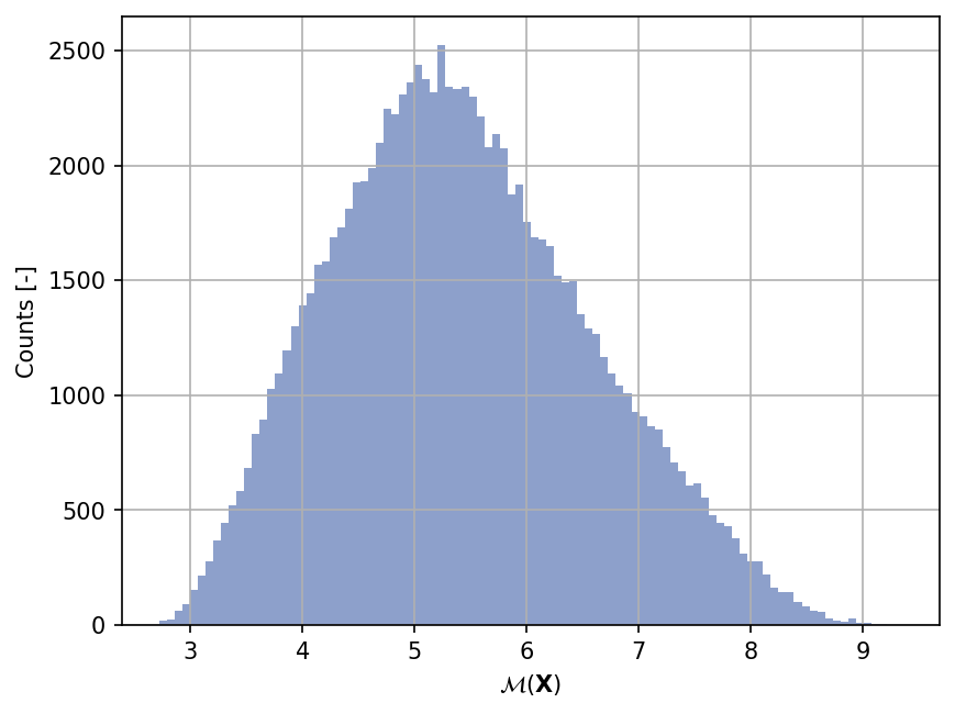
Sample histogram#
Shown below is the histogram of the output based on \(100'000\) random points:
Moments estimation#
Shown below is the convergence of a direct Monte-Carlo estimation of the output mean and variance with increasing sample sizes.
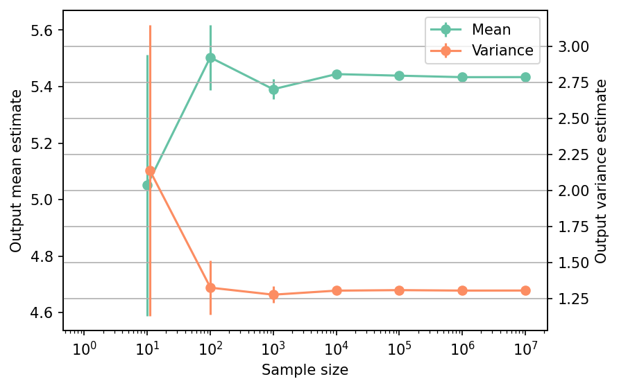
The tabulated results for is shown below.
| Sample size | Mean | Mean error | Variance | Variance error | Remark |
|---|---|---|---|---|---|
| 10 | 5.0512 | 4.6256e-01 | 2.1396 | 1.0086e+00 | Monte-Carlo |
| 100 | 5.5032 | 1.1517e-01 | 1.3264 | 1.8853e-01 | Monte-Carlo |
| 1000 | 5.3907 | 3.5747e-02 | 1.2779 | 5.7176e-02 | Monte-Carlo |
| 10000 | 5.4441 | 1.1427e-02 | 1.3058 | 1.8468e-02 | Monte-Carlo |
| 100000 | 5.4386 | 3.6186e-03 | 1.3094 | 5.8558e-03 | Monte-Carlo |
| 1000000 | 5.4333 | 1.1429e-03 | 1.3062 | 1.8473e-03 | Monte-Carlo |
| 10000000 | 5.4335 | 3.6147e-04 | 1.3066 | 5.8433e-04 | Monte-Carlo |
References#
Hyejung Moon. Design and analysis of computer experiments for screening input variables. PhD thesis, Ohio State University, Ohio, 2010. URL: http://rave.ohiolink.edu/etdc/view?acc_num=osu1275422248.
Einat Neumann Ben-Ari and David M. Steinberg. Modeling data from computer experiments: an empirical comparison of kriging with MARS and projection pursuit regression. Quality Engineering, 19(4):327–338, 2007. doi:10.1080/08982110701580930.