Two-dimensional (2D) Cantilever Beam Reliability Problem#
import numpy as np
import matplotlib.pyplot as plt
import uqtestfuns as uqtf
The 2D cantilever beam problem is a reliability test function from [RE93]. This is an often revisited problem in reliability analysis (see, for instance, [LGG+18]).
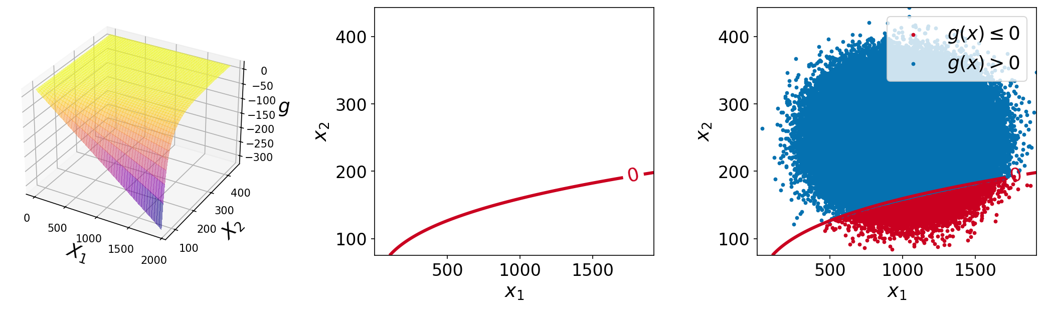
The plots of the function are shown below. The left plot shows the surface plot of the performance function, the center plot shows the contour plot with a single contour line at function value of \(0.0\) (the limit-state surface), and the right plot shows the same plot with \(10^6\) sample points overlaid.
Test function instance#
To create a default instance of the test function:
my_testfun = uqtf.CantileverBeam2D()
Check if it has been correctly instantiated:
print(my_testfun)
Function ID      : CantileverBeam2D
Input Dimension  : 2 (fixed)
Output Dimension : 1
Parameterized    : True
Description      : Cantilever beam reliability problem from Rajashekhar and Ellington (1993)
Applications     : reliability
Description#
The problem consists of a cantilever beam with a rectangular cross-section subjected to a uniformly distributed loading. The maximum deflection at the free end is taken to be the performance criterion and the performance function reads[1]:
where \(I\), the moment inertia of the cross-section, is given as follows:
By plugging in the above expression to the performance function, the following expression for the performance function is obtained:
where \(\boldsymbol{x} = \{ w, h \}\) is the two-dimensional vector of input variables, namely the load per unit area and the depth of the cross-section. These inputs are probabilistically defined further below.
The parameters of the test function \(\boldsymbol{p} = \{ E, l \}\), namely the beam’s modulus of elasticity (\(E\)) and the span of the beam (\(l\)). The values for these parameters can be found the subsequent section.
The failure state and the failure probability are defined as \(g(\boldsymbol{x}; \boldsymbol{p}) \leq 0\) and \(\mathbb{P}[g(\boldsymbol{X}; \boldsymbol{p}) \leq 0]\), respectively.
Probabilistic input#
Based on [RE93], the probabilistic input model for the test function consists of two independent standard normal random variables (see the table below).
Function ID     : Cantilever2D
Input ID        : Rajashekhar1993
Input Dimension : 2
Description     : Input model for the cantilever beam problem from
                  Rajashekhar and Ellingwood (1993)
Marginals       :

 No.    Name    Distribution    Parameters              Description
-----  ------  --------------  -------------  -------------------------------
  1      W         normal      [1000.  200.]    Load per unit area [N/m^2]
  2      H         normal      [250.   37.5]  Depth of the cross-section [mm]

Copulas         : Independence
Parameters#
The default values of the parameters are shown below.
Function ID  : CantileverBeam2D
Parameter ID : Rajashekhar1993
Description  : Parameter set for the 2D cantilever beam problem from
               Rajashekhar and Ellingwood (1993)

 No.    Keyword      Value      Type             Description
-----  ---------  -----------  ------  -------------------------------
  1     modulus   2.60000e+04  float   Modulus of elasticity 'E' [MPa]
  2      span     6.00000e+03  float      Span of the beam 'l' [mm]
Reference results#
This section provides several reference results of typical UQ analyses involving the test function.
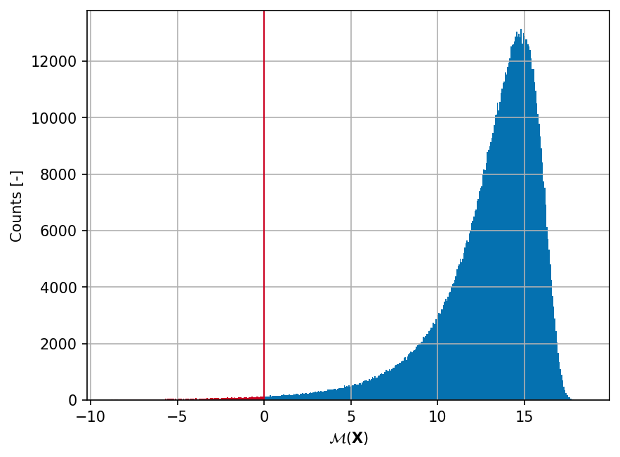
Sample histogram#
Shown below is the histogram of the output based on \(10^6\) random points:
Failure probability (\(P_f\))#
Some reference values for the failure probability \(P_f\) from the literature are summarized in the table below.
Method |
\(N\) |
\(\hat{P}_f\) |
\(\mathrm{CoV}[\hat{P}_f]\) |
Source |
Remark |
|---|---|---|---|---|---|
\(10^6\) |
\(9.594 \times 10^{-3}\) |
— |
[LGG+18] |
— |
|
\(27\) |
\(9.88 \times 10^{-3}\) |
— |
[LGG+18] |
— |
|
— |
\(9.9031 \times 10^{-3}\) |
— |
[RE93] |
— |
|
\(32\) |
\(9.88 \times 10^{-3}\) |
— |
[LGG+18] |
— |
|
\(10^3\) |
\(9.6071 \times 10^{-3}\) |
— |
[RE93] |
Importance Sampling (IS) |
|
\(9'312\) |
\(1.00 \times 10^{-2}\) |
— |
[SG05] |
— |
|
IS + RS |
\(2'192\) |
\(9.00 \times 10^{-3}\) |
— |
[SG05] |
IS + Response Surface (RS) |
IS + SP |
\(358\) |
\(1.00 \times 10^{-2}\) |
— |
[SG05] |
IS + Splines (SP) |
IS + NN |
\(63\) |
\(1.20 \times 10^{-2}\) |
— |
[SG05] |
IS + Neural Networks (NN) |
DS |
\(551\) |
\(1.000 \times 10^{-2}\) |
— |
[SG05] |
Directional sampling (DS) |
DS + RS |
\(60\) |
\(6.00 \times 10^{-3}\) |
— |
[SG05] |
DS + Response Surface (RS) |
DS + SP |
\(57\) |
\(7.00 \times 10^{-3}\) |
— |
[SG05] |
DS + Splines (SP |
DS + NN |
\(40\) |
\(8.00 \times 10^{-3}\) |
— |
[SG05] |
DS + Neural Networks (NN) |
SSRM |
\(18\) |
\(9.499 \times 10^{-3}\) |
— |
[LGG+18] |
Sequential surrogate reliability method |
Bucher’s |
— |
\(1.37538 \times 10^{-2}\) |
— |
[RE93] |
— |
Approach A-0 |
— |
\(9.5410 \times 10^{-3}\) |
— |
[RE93] |
— |
Approach A-1 |
— |
\(9.6398 \times 10^{-3}\) |
— |
[RE93] |
— |
Approach A-2 |
— |
\(1.11508 \times 10^{-2}\) |
— |
[RE93] |
— |
Approach A-3 |
— |
\(9.5410 \times 10^{-3}\) |
— |
[RE93] |
— |
References#
Xu Li, Chunlin Gong, Liangxian Gu, Wenkun Gao, Zhao Jing, and Hua Su. A sequential surrogate method for reliability analysis based on radial basis function. Structural Safety, 73:42–53, 2018. doi:10.1016/j.strusafe.2018.02.005.