Borehole Function#
import numpy as np
import matplotlib.pyplot as plt
import uqtestfuns as uqtf
The Borehole test function is an eight-dimensional scalar-valued function. The function has been used in the context of sensitivity analysis [HG83, Wor87] and metamodeling [MMY93].
Test function instance#
To create a default instance of the Borehole test function:
my_testfun = uqtf.Borehole()
Check if it has been correctly instantiated:
print(my_testfun)
Function ID      : Borehole
Input Dimension  : 8 (fixed)
Output Dimension : 1
Parameterized    : False
Description      : Borehole function from Harper and Gupta (1983)
Applications     : metamodeling, sensitivity
Description#
The Borehole function models the flow rate of water through a borehole drilled from the ground surface through two aquifers. The model assumes laminar-isothermal flow, and there is no groundwater gradient, with steady-state flow between the upper aquifer and the borehole and between the borehole and the lower aquifer [HG83]. The function computes the water flow rate through the borehole using the following analytical formula:
where \(\boldsymbol{x} = \{ r_w, r, T_u, H_u, T_l, H_l, L, K_w\}\) is the vector of input variables defined below. The unit of the output is \(\left[ \mathrm{m}^3 / \mathrm{year} \right]\).
Probabilistic input#
There are two probabilistic input models available as shown in the table below.
In both specifications, the input variables are modeled as independent random variables. The marginals of the original specification (from [HG83]) are shown below:
Function ID     : Borehole
Input ID        : Harper1983
Input Dimension : 8
Description     : Probabilistic input model of the Borehole model from
                  Harper and Gupta (1983)
Marginals       :

 No.    Name    Distribution        Parameters                          Description
-----  ------  --------------  ---------------------  -----------------------------------------------
  1      rw        normal      [0.1       0.0161812]            radius of the borehole [m]
  2      r       lognormal        [7.71   1.0056]                 radius of influence [m]
  3      Tu       uniform        [ 63070. 115600.]      transmissivity of upper aquifer [m^2/year]
  4      Hu       uniform          [ 990. 1100.]         potentiometric head of upper aquifer [m]
  5      Tl       uniform          [ 63.1 116. ]        transmissivity of lower aquifer [m^2/year]
  6      Hl       uniform           [700. 820.]          potentiometric head of lower aquifer [m]
  7      L        uniform          [1120. 1680.]                length of the borehole [m]
  8      Kw       uniform         [ 9985. 12045.]     hydraulic conductivity of the borehole [m/year]

Copulas         : Independence
Note
In [MMY93], the non-uniform distributions (\(r_w\) and \(r\)) are replaced with uniform distributions.
For example, to create a Borehole test function using the input specification by [MMY93]:
my_testfun = uqtf.Borehole(input_id="Morris1993")
Reference results#
This section provides several reference results of typical UQ analyses involving the test function.
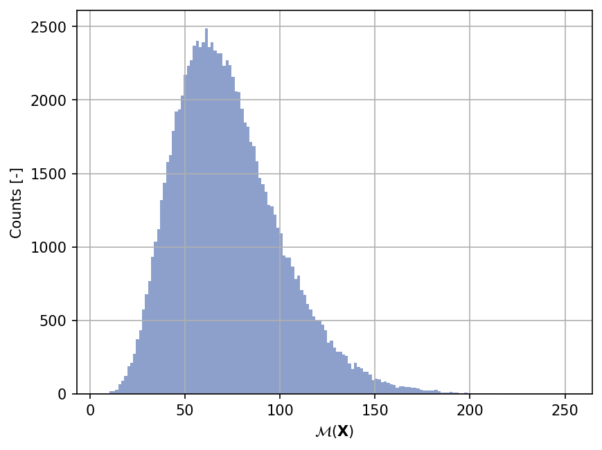
Sample histogram#
Shown below is the histogram of the output based on \(100'000\) random points:
Moments estimation#
Shown below is the convergence of a direct Monte-Carlo estimation of the output mean and variance with increasing sample sizes.
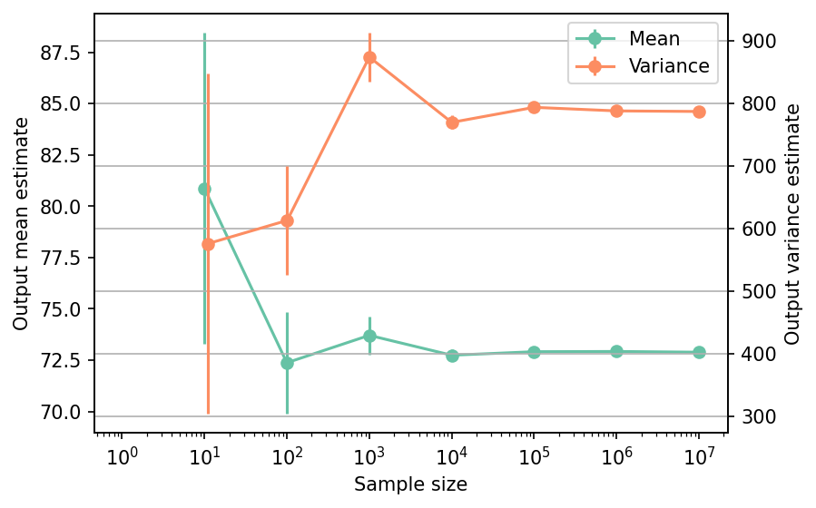
The tabulated results for each sample size is shown below.
| Sample size | Mean | Mean error | Variance | Variance error | Remark |
|---|---|---|---|---|---|
| 10 | 8.0877e+01 | 7.5904e+00 | 5.7614e+02 | 2.7159e+02 | Monte-Carlo |
| 100 | 7.2374e+01 | 2.4766e+00 | 6.1334e+02 | 8.7176e+01 | Monte-Carlo |
| 1000 | 7.3710e+01 | 9.3517e-01 | 8.7454e+02 | 3.9130e+01 | Monte-Carlo |
| 10000 | 7.2741e+01 | 2.7750e-01 | 7.7007e+02 | 1.0891e+01 | Monte-Carlo |
| 100000 | 7.2913e+01 | 8.9112e-02 | 7.9410e+02 | 3.5513e+00 | Monte-Carlo |
| 1000000 | 7.2924e+01 | 2.8079e-02 | 7.8840e+02 | 1.1150e+00 | Monte-Carlo |
| 10000000 | 7.2888e+01 | 8.8741e-03 | 7.8749e+02 | 3.5218e-01 | Monte-Carlo |
References#
William V. Harper and Sumant K. Gupta. Sensitivity/uncertainty analysis of a borehole scenario comparing latin hypercube sampling and deterministic sensitivity approaches. Technical Report BMI/ONWI-516, Office of Nuclear Waste Isolation, Battelle Memorial Institute, 1983. URL: https://inldigitallibrary.inl.gov/PRR/84393.pdf.
Brian A. Worley. Deterministic uncertainty analysis. Technical Report ORNL-6428, Oak Ridge National Laboratory (ORNL), Oak Ridge, Tennessee, 1987. doi:10.2172/5534706.
Max D. Morris, T. J. Mitchell, and D. Ylvisaker. Bayesian design and analysis of computer experiments: use of derivatives in surface prediction. Technometrics, 35(3):245–255, 1993. doi:10.1080/00401706.1993.10485320.