Tutorial: Test a Reliability Analysis Method#
UQTestFuns includes several test functions from the literature employed in a reliability analysis exercise. In this tutorial, you’ll implement a method to estimate the failure probability of a computational model and test the implementation using a test function available in UQTestFuns.
By the end of this tutorial, you’ll get an idea how a function from UQTestFuns is used to test a reliability analysis method.
import numpy as np
import matplotlib.pyplot as plt
import uqtestfuns as uqtf
Reliability analysis#
Consider a system whose performance is defined by a performance function[1] \(g\) whose values, in turn, depend on:
\(\boldsymbol{x}_p\): the (uncertain) input variables of an underlying computational model \(\mathcal{M}\)
\(\boldsymbol{x}_s\): additional (uncertain) input variables that affects the performance of the system, but not part of inputs to \(\mathcal{M}\)
\(\boldsymbol{p}\): an additional set of deterministic parameters of the system
Combining these variables and parameters as an input to the performance function \(g\):
where \(\boldsymbol{x} = \{ \boldsymbol{x}_p, \boldsymbol{x}_s \}\).
The system is said to be in failure state if and only if \(g(\boldsymbol{x}; \boldsymbol{p}) \leq 0\); the set of all values \(\{ \boldsymbol{x}, \boldsymbol{p} \}\) such that \(g(\boldsymbol{x}; \boldsymbol{p}) \leq 0\) is called the failure domain.
Conversely, the system is said to be in safe state if and only if \(g(\boldsymbol{x}; \boldsymbol{p}) > 0\); the set of all values \(\{ \boldsymbol{x}, \boldsymbol{p} \}\) such that \(g(\boldsymbol{x}; \boldsymbol{p}) > 0\) is called the safe domain.
Failure probability#
Reliability analysis[2] concerns with estimating the failure probability of a system with a given performance function \(g\). For a given joint probability density function (PDF) \(f_{\boldsymbol{X}}\) of the uncertain input variables \(\boldsymbol{X} = \{ \boldsymbol{X}_p, \boldsymbol{X}_s \}\), the failure probability \(P_f\) of the system is defined as follows [Sud12, VAK15]:
Evaluating the above integral is, in general, non-trivial because the domain of integration is only provided implicitly and the number of dimensions may be large.
Monte-Carlo estimation#
Warning
The Monte-Carlo method implemented below is one of the most straightforward and robust approach to estimate (small) failure probability. However, the method is rarely used for practical applications due to its high computational cost. It is used here in this tutorial simply as an illustration. Numerous methods have been developed to efficiently and accurately estimate the failure probability of a computational model.
The failure probability of a computational model given probabilistic inputs may be directly estimated using a Monte-Carlo simulation. Such a method is straightforward to implement though potentially computationally expensive as the chance of observing a failure event in a typical reliability analysis problem is very small.
An alternative formulation of the failure probability following [BZ15] that aligns well with Monte-Carlo simulation is given below:
where \(\mathbb{I}[g(\boldsymbol{x}; \boldsymbol{p}) \leq 0]\) is the indicator function such that:
The Monte-Carlo estimate of the failure probability is given as follows:
where \(N\) is the number of Monte-Carlo sample points.
To assess the accuracy of the estimate given by the above equation, the coefficient of variation (\(\mathrm{CoV}\)) is often used:
The Monte-Carlo simulation method to estimate the failure probability is summarized in Algorithm 4.
Algorithm 4 (Monte-Carlo simulation for estimating \(P_f\))
Inputs A performance function \(g\), random input variables \(\boldsymbol{X}\), number of MC sample points \(N\)
Output \(\widehat{P}_f\) and \(\mathrm{CoV}[\widehat{P}_f]\)
\(N_f \leftarrow 0\)
For \(i = 1\) to \(N\):
Sample \(\boldsymbol{x}^{(i)}\) from \(\boldsymbol{X}\)
Evaluate \(g(\boldsymbol{x}^{(i); \boldsymbol{p}})\)
If \(g(\boldsymbol{x}^{(i)}; \boldsymbol{p}) \leq 0\):
\(N_f \leftarrow N_f + 1\)
\(\widehat{P}_f = \frac{N_f}{N}\)
\(\mathrm{CoV}[\widehat{P}_f] = \left( \frac{1 - \widehat{P}_f}{N \widehat{P}_f} \right)^{0.5}\)
Algorithm 4 is implemented in a Python function that assumes the performance function can be evaluated in a vectorized manner and a probabilistic model of the relevant inputs has been defined such that sample points can be generated from them.
Note
And indeed, test functions included in UQTestFuns are all given with the corresponding probabilistic input model according to the literature.
Two-dimensional cantilever beam reliability problem#
To test the implemented algorithm above, we choose the two-dimensional cantilever beam reliability problem included in UQTestFuns. Several published results are available for this problem.
The reliability problem consists of a cantilever beam with a rectangular cross-section subjected to a uniformly distributed loading. The maximum deflection at the free end is taken to be the performance criterion such that the performance function reads:
where \(\boldsymbol{x} = \{ w, h \}\) is the two-dimensional vector of input variables, namely the load per unit area (\(w\)) and the depth of the cross section (\(h\)); and \(\boldsymbol{p} = \{ E l\}\) is the vector of parameters, namely the modulus of elasticity of the beam (\(E\)) and the span of the beam (\(l\)).
To create an instance of the cantilever beam function:
cantilever = uqtf.CantileverBeam2D()
The input variables \(w\) and \(h\) are probabilistically defined according to the table below.
print(cantilever.prob_input)
Function ID     : Cantilever2D
Input ID        : Rajashekhar1993
Input Dimension : 2
Description     : Input model for the cantilever beam problem from
                  Rajashekhar and Ellingwood (1993)
Marginals       :

 No.    Name    Distribution    Parameters              Description
-----  ------  --------------  -------------  -------------------------------
  1      W         normal      [1000.  200.]    Load per unit area [N/m^2]
  2      H         normal      [250.   37.5]  Depth of the cross-section [mm]

Copulas         : Independence
The default values of the parameters \(E\) and \(l\) are:
print(cantilever.parameters)
Function ID  : CantileverBeam2D
Parameter ID : Rajashekhar1993
Description  : Parameter set for the 2D cantilever beam problem from
               Rajashekhar and Ellingwood (1993)

 No.    Keyword      Value      Type             Description
-----  ---------  -----------  ------  -------------------------------
  1     modulus   2.60000e+04  float   Modulus of elasticity 'E' [MPa]
  2      span     6.00000e+03  float      Span of the beam 'l' [mm]
For reproducibility of this tutorial, set the seed number of the pseudo-random generator attached to the probabilistic input model:
cantilever.prob_input.reset_rng(245634)
Finally, several published results of the failure probability of the problem are as follows:
\(\widehat{P}_f = 9.88 \times 10^{-3}\) using FORM with \(27\) performance function evaluations ([LGG+18])
\(\widehat{P}_f = 9.6071 \times 10^{-3}\) using IS with \(10^3\) performance function evaluations ([RE93])
\(\widehat{P}_f = 9.499 \times 10^{-3}\) using sequential surrogate reliability method with \(18\) performance function evaluations ([LGG+18])
Failure probability estimation#
To observe the convergence of the estimation procedure implemented above, several Monte-Carlo sample sizes are used:
sample_sizes = 5**np.arange(3, 12)
pf_estimates = np.zeros(len(sample_sizes))
cov_estimates = np.zeros(len(sample_sizes))

for i, sample_size in enumerate(sample_sizes):
    pf_estimates[i], cov_estimates[i] = estimate_pf(
        cantilever, cantilever.prob_input, sample_size
    )
The estimated failure probability as a function of sample size is plotted below. The uncertainty band around the estimate is also included and it corresponds to one standard deviation.
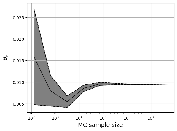
The final estimate of the failure probability (from \(>10^7\) function evaluations) is:
print(f"{pf_estimates[-1]:1.4e}")
9.5340e-03
This values seems to be consistent with the provided published results albeit with a much higher computational cost.
The challenge for a reliability analysis method is to accurately and efficiently (as few performance function evaluations as possible) estimate the failure probability.
References#
Bruno Sudret. Meta-models for structural reliability and uncertainty quantification. In Proceedings of the 5th Asian-Pacific Symposium on Structural Reliability and its Applications. 2012. doi:10.3850/978-981-07-2219-7_p321.
Ajit Kumar Verma, Srividya Ajit, and Durga Rao Karanki. Structural reliability. In Springer Series in Reliability Engineering, pages 257–292. Springer London, 2015. doi:10.1007/978-1-4471-6269-8_8.
James L. Beck and Konstantin M. Zuev. Rare-event simulation. In Handbook of Uncertainty Quantification, pages 1–26. Springer International Publishing, 2015. doi:10.1007/978-3-319-11259-6_24-1.
Xu Li, Chunlin Gong, Liangxian Gu, Wenkun Gao, Zhao Jing, and Hua Su. A sequential surrogate method for reliability analysis based on radial basis function. Structural Safety, 73:42–53, 2018. doi:10.1016/j.strusafe.2018.02.005.
Malur R. Rajashekhar and Bruce R. Ellingwood. A new look at the response surface approach for reliability analysis. Structural Safety, 12(3):205–220, 1993. doi:10.1016/0167-4730(93)90003-j.