Convex Failure Domain Reliability Problem#

import numpy as np
import matplotlib.pyplot as plt
import uqtestfuns as uqtf

The Convex failure domain is a test function from [BS97] for reliability analysis exercises [Waa00].

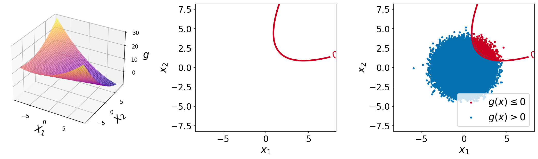
The plots of the function are shown below. The left plot shows the surface plot of the performance function, the center plot shows the contour plot with a single contour line at function value of \(0.0\) (the limit-state surface), and the right plot shows the same plot with \(10^6\) sample points overlaid.

Test function instance#

To create a default instance of the test function:

my_testfun = uqtf.ConvexFailDomain()

Check if it has been correctly instantiated:

print(my_testfun)

Name              : ConvexFailDomain
Spatial dimension : 2
Description       : Convex failure domain problem from Borri and Speranzini (1997)

Description#

The test function (i.e., the performance function) is analytically defined as follows:

\[ g(\boldsymbol{x}) = 0.1 (x_1 - x_2)^2 - \frac{(x_1 + x_2)}{\sqrt{2}} + 2.5, \]

where \(\boldsymbol{x} = \{ x_1, x_2 \}\) is the two-dimensional vector of input variables probabilistically defined further below.

The failure state and the failure probability are defined as \(g(\boldsymbol{x}) \leq 0\) and \(\mathbb{P}[g(\boldsymbol{X}) \leq 0]\), respectively.

Probabilistic input#

Based on [BS97], the probabilistic input model for the test function consists of two independent standard normal random variables (see the table below).

my_testfun.prob_input

Name: ConvexFailDomain-Borri1997

Spatial Dimension: 2

Description: Input model for the convex failure domain problem from Borri and Speranzini (1997)

Marginals:

No.	Name	Distribution	Parameters	Description
1	X1	normal	[0 1]	None
2	X2	normal	[0 1]	None

Copulas: None

Reference results#

This section provides several reference results of typical UQ analyses involving the test function.

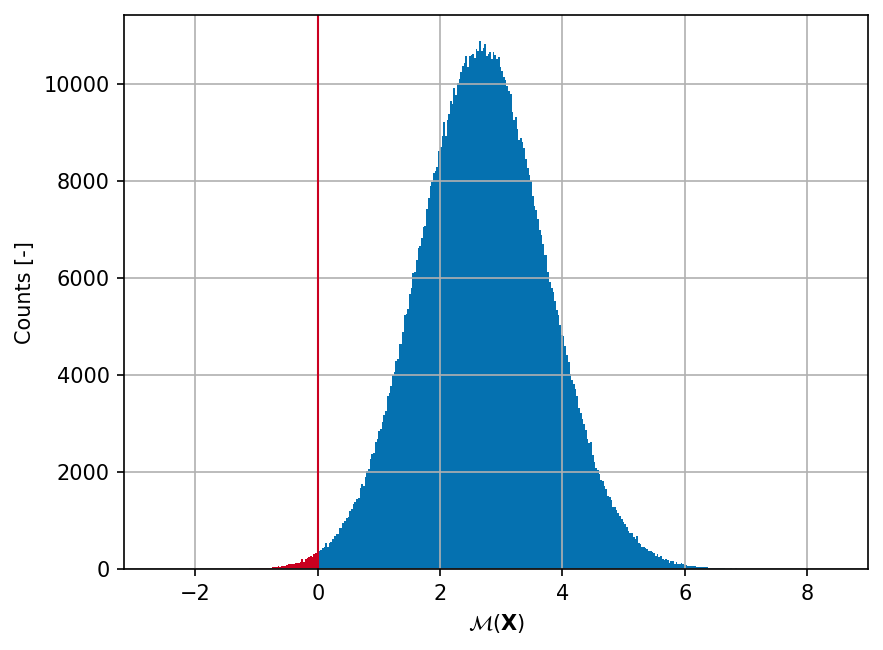
Sample histogram#

Shown below is the histogram of the output based on \(10^6\) random points:

def is_outlier(points, thresh=3.5):
    """
    Returns a boolean array with True if points are outliers and False 
    otherwise.

    This is taken from:
    https://stackoverflow.com/questions/11882393/matplotlib-disregard-outliers-when-plotting
    
    Parameters:
    -----------
        points : An numobservations by numdimensions array of observations
        thresh : The modified z-score to use as a threshold. Observations with
            a modified z-score (based on the median absolute deviation) greater
            than this value will be classified as outliers.

    Returns:
    --------
        mask : A numobservations-length boolean array.

    References:
    ----------
        Boris Iglewicz and David Hoaglin (1993), "Volume 16: How to Detect and
        Handle Outliers", The ASQC Basic References in Quality Control:
        Statistical Techniques, Edward F. Mykytka, Ph.D., Editor. 
    """
    if len(points.shape) == 1:
        points = points[:,None]
    median = np.median(points, axis=0)
    diff = np.sum((points - median)**2, axis=-1)
    diff = np.sqrt(diff)
    med_abs_deviation = np.median(diff)

    modified_z_score = 0.6745 * diff / med_abs_deviation

    return modified_z_score > thresh

xx_test = my_testfun.prob_input.get_sample(1000000)
yy_test = my_testfun(xx_test)
yy_test = yy_test[~is_outlier(yy_test, thresh=10)]
idx_pos = yy_test > 0
idx_neg = yy_test <= 0

hist_pos = plt.hist(yy_test, bins="auto", color="#0571b0")
plt.hist(yy_test[idx_neg], bins=hist_pos[1], color="#ca0020")
plt.axvline(0, linewidth=1.0, color="#ca0020")

plt.grid()
plt.ylabel("Counts [-]")
plt.xlabel("$\mathcal{M}(\mathbf{X})$")
plt.gcf().set_dpi(150);

Failure probability (\(P_f\))#

Some reference values for the failure probability \(P_f\) from the literature are summarized in the table below.

Method	\(N\)	\(\hat{P}_f\)	\(\mathrm{CoV}[\hat{P}_f]\)	Source	Remark
Exact	—	\(4.2692 \times 10^{-3}\)	—	[Waa00]	Annex E.6 Table: Results
FORM	\(8\)	\(6.2097 \times 10^{-3}\)	—	[Waa00]	Annex E.6 Table: Results
MCS	\(10^{4}\)	\(4.2692 \times 10^{-3}\)	\(0.02\)	[Waa00]	Annex E.6 Table: Results

References#

BS97(1,2): Antonio Borri and Emanuela Speranzini. Structural reliability analysis using a standard deterministic finite element code. Structural Safety, 19(4):361–382, 1997. doi:10.1016/s0167-4730(97)00017-9.
Waa00(1,2,3,4): Paul Hendrik Waarts. Structural reliability using finite element analysis - an appraisal of DARS: Directional adaptive response surface sampling. phdthesis, Civil Engineering and Geosciences, TU Delt, Delft, The Netherlands, 2000. URL: https://repository.tudelft.nl/islandora/object/uuid:6e6d9a76-fd12-4220-9dc1-36515b3f638d.

UQTestFuns

Convex Failure Domain Reliability Problem

Contents