Ackley Function#
The Ackley function is an \(M\)-dimensional scalar-valued function. Introduced by Ackley [Ack87] as a benchmark function for global optimization algorithms, the function was originally presented in two dimensions. Bäck and Schwefel [BS93] later generalized the function to higher dimensions. More recently, it was employed as a test function for a metamodeling method in [KSC+17].
import numpy as np
import matplotlib.pyplot as plt
import uqtestfuns as uqtf
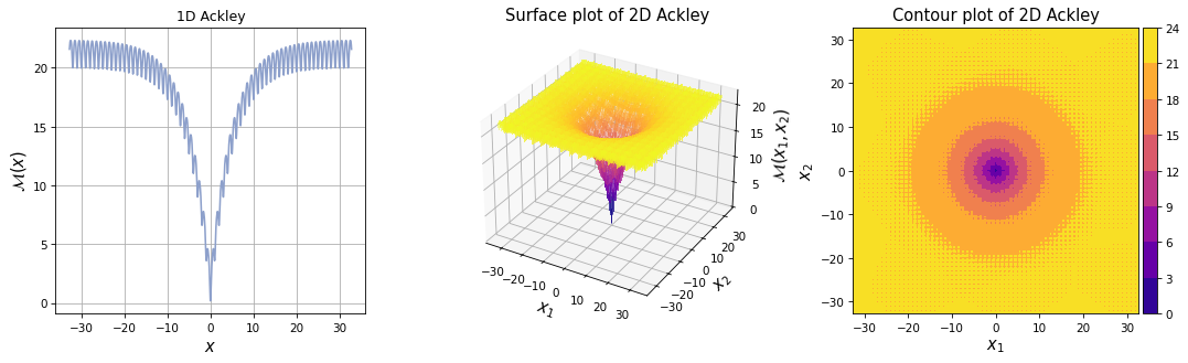
The plots for one-dimensional and two-dimensional Ackley function are shown below. As can be seen, the function features many local optima with a single global optima.
Test function instance#
To create a default instance of the Ackley test function, type:
my_testfun = uqtf.Ackley()
Check if it has been correctly instantiated:
print(my_testfun)
Function ID      : Ackley
Input Dimension  : 2 (variable)
Output Dimension : 1
Parameterized    : True
Description      : Optimization test function from Ackley (1987)
Applications     : optimization, metamodeling
By default, the input dimension is set to \(2\)[1].
To create an instance with another value of input dimension,
pass an integer to the parameter input_dimension (keyword only).
For example, to create an instance of 10-dimensional Ackley function, type:
my_testfun = uqtf.Ackley(input_dimension=10)
In the subsequent section, this 10-dimensional Ackley function will be used for illustration.
Description#
The generalized Ackley function according to [BS93] is defined as follows:
where \(\boldsymbol{x} = \{ x_1, \ldots, x_M \}\) is the \(M\)-dimensional vector of input variables further defined below, and \(\boldsymbol{a} = \{ a_1, a_2, a_3 \}\) are parameters of the function.
Input#
Based on [Ack87], the search domain of the Ackley function is in \([-32.768, 32.768]^M\). In UQTestFuns, this search domain can be represented as probabilistic input using the uniform distribution with marginals shown in the table below.
Function ID     : Ackley
Input ID        : Ackley1987
Input Dimension : 10
Description     : Search domain for the Ackley function from Ackley (1987)
Marginals       :

 No.    Name    Distribution      Parameters       Description
-----  ------  --------------  -----------------  -------------
  1      X1       uniform      [-32.768  32.768]        -
  2      X2       uniform      [-32.768  32.768]        -
  3      X3       uniform      [-32.768  32.768]        -
  4      X4       uniform      [-32.768  32.768]        -
  5      X5       uniform      [-32.768  32.768]        -
  6      X6       uniform      [-32.768  32.768]        -
  7      X7       uniform      [-32.768  32.768]        -
  8      X8       uniform      [-32.768  32.768]        -
  9      X9       uniform      [-32.768  32.768]        -
 10     X10       uniform      [-32.768  32.768]        -

Copulas         : Independence
Parameters#
The Ackley function requires three additional parameters to complete the specification. The default values are shown below.
Function ID  : Ackley
Parameter ID : Ackley1987
Description  : Parameter set for the Ackley function from Ackley (1987)

 No.    Keyword      Value      Type                   Description
-----  ---------  -----------  ------  --------------------------------------------
  1        a      2.00000e+01  float   Height of the ridges surrounding the minimum
  2        b      2.00000e-01  float       Decay rate of the Euclidean distance
  3        c      6.28319e+00  float       Scaling constant for the cosine term
Reference results#
This section provides several reference results related to the test function.
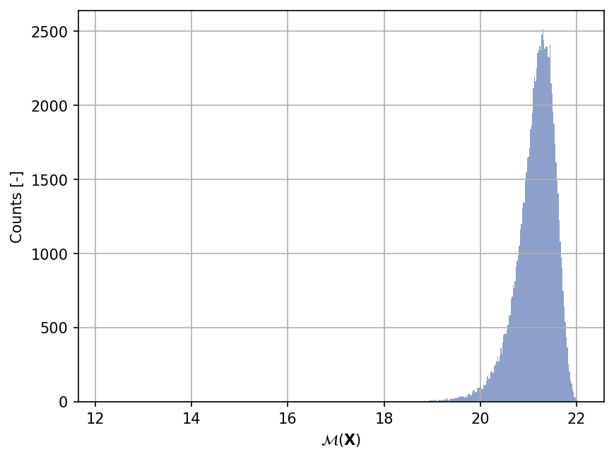
Sample histogram#
Shown below is the histogram of the output based on \(100'000\) random points:
Optimum values#
The global optimum value of the Ackley function is \(\mathcal{M}(\boldsymbol{x}^*) = 0\) at \(x_m^* = 0,\, m = 1, \ldots, M\).
References#
David H. Ackley. A connectionist machine for genetic hillclimbing. The Springer International Series in Engineering and Computer Science (SECS, volume 28). Springer US, Boston, MA., 1987. doi:10.1007/978-1-4613-1997-9.
Thomas Bäck and Hans-Paul Schwefel. An overview of evolutionary algorithms for parameter optimization. Evolutionary Computation, 1(1):1–23, 1993. doi:10.1162/evco.1993.1.1.1.
A. Kaintura, D. Spina, I. Couckuyt, L. Knockaert, W. Bogaerts, and T. Dhaene. A Kriging and Stochastic Collocation ensemble for uncertainty quantification in engineering applications. Engineering with Computers, 33(4):935–949, 2017. doi:10.1007/s00366-017-0507-0.