Circular Bar RS Reliability Problem#

import numpy as np
import matplotlib.pyplot as plt
import uqtestfuns as uqtf

The circular bar RS reliability problem from [VAK15] is a variation on a theme of the classic RS reliability problem. This particular variant put it in the context of a circular bar subjected to an axial force.

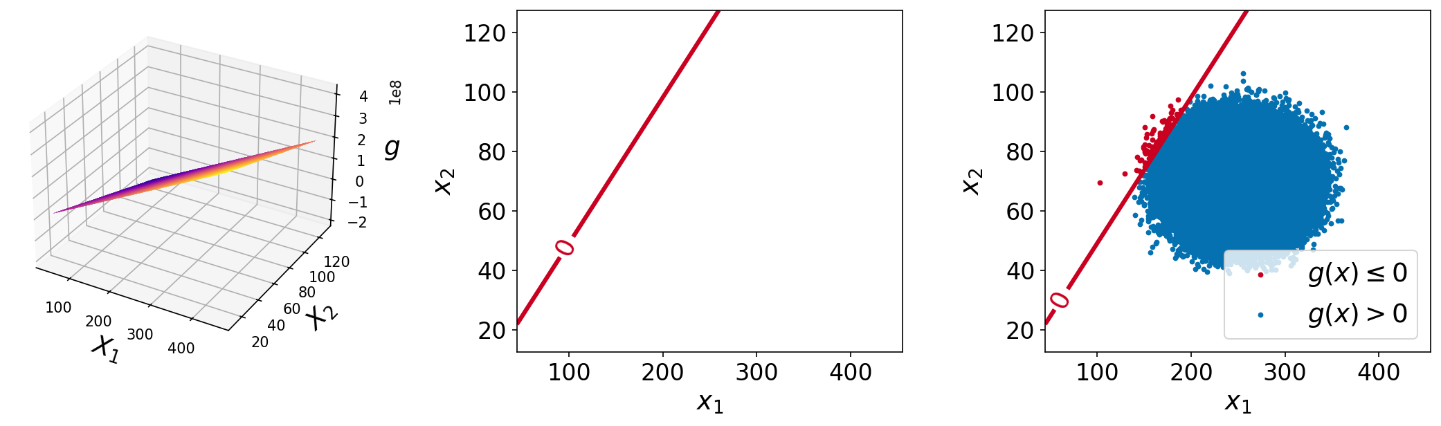
The plots of the function are shown below. The left plot shows the surface plot of the performance function, the center plot shows the contour plot with a single contour line at function value of \(0.0\) (the limit-state surface), and the right plot shows the same plot with \(10^6\) sample points overlaid.

Test function instance#

To create a default instance of the test function:

my_testfun = uqtf.RSCircularBar()

Check if it has been correctly instantiated:

print(my_testfun)

Name              : RSCircularBar
Spatial dimension : 2
Description       : RS problem as a circular bar from Verma et al. (2016)

Description#

The reliability problem consists of a carbon-steel circular bar subjected to an axial force. The test function (i.e., the performance function) is analytically defined as follows1:

\[ g(\boldsymbol{x}; p) = Y - \frac{F}{\frac{1}{4} \pi d^2}, \]

where \(\boldsymbol{x} = \{ Y, F \}\) is the two-dimensional vector of input variables probabilistically defined further below; and \(p = \{ d \}\) is the deterministic parameter of the function.

The failure state and the failure probability are defined as \(g(\boldsymbol{x}; p) \leq 0\) and \(\mathbb{P}[g(\boldsymbol{X}; p) \leq 0]\), respectively.

Probabilistic input#

Based on [VAK15], the probabilistic input model for the test function consists of two independent standard normal random variables (see the table below).

my_testfun.prob_input

Name: RSCircularBar-Verma2016

Spatial Dimension: 2

Description: Input model for the circular bar RS from Verma et al. (2016)

Marginals:

No.	Name	Distribution	Parameters	Description
1	Y	normal	[250. 25.]	Material mean yield strength [MPa]
2	F	normal	[70. 7.]	Force mean value [kN]

Copulas: None

Parameter#

The parameter of the function is \(d\) which from [VAK15] is set to \(25\;\mathrm{[mm]}\).

Reference results#

This section provides several reference results of typical UQ analyses involving the test function.

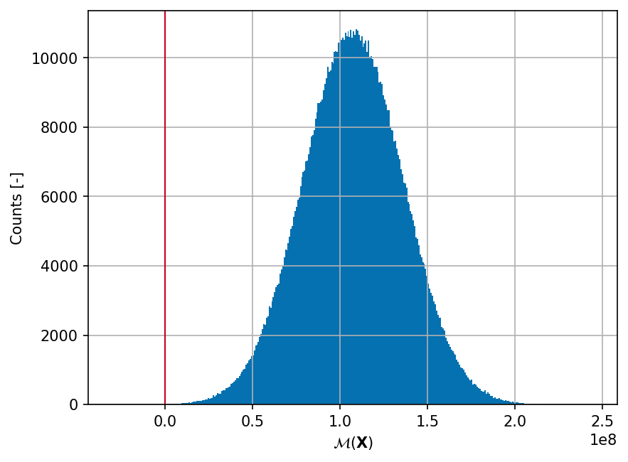
Sample histogram#

Shown below is the histogram of the output based on \(10^6\) random points:

def is_outlier(points, thresh=3.5):
    """
    Returns a boolean array with True if points are outliers and False 
    otherwise.

    This is taken from:
    https://stackoverflow.com/questions/11882393/matplotlib-disregard-outliers-when-plotting
    
    Parameters:
    -----------
        points : An numobservations by numdimensions array of observations
        thresh : The modified z-score to use as a threshold. Observations with
            a modified z-score (based on the median absolute deviation) greater
            than this value will be classified as outliers.

    Returns:
    --------
        mask : A numobservations-length boolean array.

    References:
    ----------
        Boris Iglewicz and David Hoaglin (1993), "Volume 16: How to Detect and
        Handle Outliers", The ASQC Basic References in Quality Control:
        Statistical Techniques, Edward F. Mykytka, Ph.D., Editor. 
    """
    if len(points.shape) == 1:
        points = points[:,None]
    median = np.median(points, axis=0)
    diff = np.sum((points - median)**2, axis=-1)
    diff = np.sqrt(diff)
    med_abs_deviation = np.median(diff)

    modified_z_score = 0.6745 * diff / med_abs_deviation

    return modified_z_score > thresh

xx_test = my_testfun.prob_input.get_sample(1000000)
yy_test = my_testfun(xx_test)
yy_test = yy_test[~is_outlier(yy_test, thresh=10)]
idx_pos = yy_test > 0
idx_neg = yy_test <= 0

hist_pos = plt.hist(yy_test, bins="auto", color="#0571b0")
plt.hist(yy_test[idx_neg], bins=hist_pos[1], color="#ca0020")
plt.axvline(0, linewidth=1.0, color="#ca0020")

plt.grid()
plt.ylabel("Counts [-]")
plt.xlabel("$\mathcal{M}(\mathbf{X})$")
plt.gcf().set_dpi(150);

Failure probability (\(P_f\))#

Some reference values for the failure probability \(P_f\) from the literature are summarized in the table below.

Method	\(N\)	\(\hat{P}_f\)	\(\mathrm{CoV}[\hat{P}_f]\)	Source	Remark
FOSM	\(12\)	\(9.4231 \times 10^{-5}\)	—	[VAK15]	\(\beta = 3.734\) (p. 261)

References#

VAK15(1,2,3,4,5): Ajit Kumar Verma, Srividya Ajit, and Durga Rao Karanki. Structural reliability. In Springer Series in Reliability Engineering, pages 257–292. Springer London, 2015. doi:10.1007/978-1-4471-6269-8_8.

1: see Example 1, Chapter 8, p. 260 in [VAK15].

UQTestFuns

Circular Bar RS Reliability Problem

Contents