Sobol’-G Function#
The Sobol’-G function is an \(M\)-dimensional scalar-valued function. It was introduced in [BFN92] for testing numerical integration algorithms (e.g., quasi-Monte-Carlo; see, for instance, [RSobolT96, Sobol98]).
The current form (and name) was from [SSobol95] and used in the context of global sensitivity analysis. There, the function was generalized by introducing a set of parameters that determines the importance of each input variable. Later on, it becomes a popular testing function for global sensitivity analysis methods; see, for instance, [SCJR22, MILR09, MIVDV08, KFSM11].
import numpy as np
import matplotlib.pyplot as plt
import uqtestfuns as uqtf
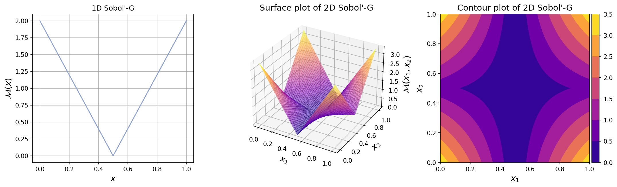
The plots for one-dimensional and two-dimensional Sobol’-G function can be seen below.
Test function instance#
To create a default instance of the Sobol’-G test function, type:
my_testfun = uqtf.SobolG()
Check if it has been correctly instantiated:
print(my_testfun)
Function ID      : SobolG
Input Dimension  : 2 (variable)
Output Dimension : 1
Parameterized    : True
Description      : Sobol'-G function from Saltelli and Sobol' (1995)
Applications     : sensitivity, integration
By default, the input dimension is set to \(2\)[1].
To create an instance with another value of input dimension,
pass an integer to the parameter input_dimension (the first parameter).
For example, to create an instance of the Sobol’-G function in six dimensions,
type:
my_testfun = uqtf.SobolG(input_dimension=6)
In the subsequent section, the function will be illustrated using six dimensions.
Description#
The Sobol’-G function is defined as follows[2]:
where \(\boldsymbol{x} = \{ x_1, \ldots, x_M \}\) is the \(M\)-dimensional vector of input variables further defined below, and \(\boldsymbol{a} = \{ a_1, \ldots, a_M \}\) are parameters of the function.
Probabilistic input#
Based on [Sobol98] the probabilistic input model for the Sobol’-G function consists of \(M\) independent uniform random variables with the ranges shown in the table below.
Function ID     : SobolG
Input ID        : Saltelli1995
Input Dimension : 6
Description     : Probabilistic input model for the Sobol'-G function from
                  Saltelli and Sobol' (1995)
Marginals       :

 No.    Name    Distribution    Parameters    Description
-----  ------  --------------  ------------  -------------
  1      X1       uniform        [0. 1.]           -
  2      X2       uniform        [0. 1.]           -
  3      X3       uniform        [0. 1.]           -
  4      X4       uniform        [0. 1.]           -
  5      X5       uniform        [0. 1.]           -
  6      X6       uniform        [0. 1.]           -

Copulas         : Independence
Parameters#
The parameters of the Sobol-G function (that is, the coefficients \(\{ a_m \}\)) determine the overall behavior of the function as well as the importance of each input variable. There are several sets of parameters used in the literature as shown in the table below.
No. |
Value |
Keyword |
Source |
Remark |
|---|---|---|---|---|
1 |
\(a_1 = \ldots = a_M = 0\) |
|
All input variables are equally important |
|
2 |
\(a_1 = a_2 = 0\) |
|
[SSobol95] (Example 2) |
The first two are important, the next is moderately important, and the rest is non-influential |
3 |
\(a_m = \frac{m - 1}{2.0}\) |
|
The most important input is the first one, the least is the last one |
|
4 |
\(a_1 = \ldots = a_M = 0.01\) |
|
[Sobol98] (choice 1) |
The supremum of the function grows exponentially at \(2^M\) |
5 |
\(a_1 = \ldots = a_M = 1.0\) |
|
[Sobol98] (choice 2) |
The supremum of the function grows exponentially at \(1.5^M\) |
6 |
\(a_m = m\) |
|
[Sobol98] (choice 3) |
The supremum of the function grows linearly at \(1 + \frac{M}{2}\) |
7 |
\(a_m = m^2\) |
|
[Sobol98] (choice 4) |
The supremum is bounded at \(1.0\) |
8 |
\(a_1 = a_2 = 0.0\) |
|
[KFSM11] (Problem 2A) |
Originally, \(M = 100\) |
9 |
\(a_m = 6.52\) |
|
[KFSM11] (Problem 3B) |
|
10 |
\(a_{1 - 4} = (0, 1, 4.5, 9)\) |
|
[SCJR22] (Section 3.2) |
Note
The parameter values used in [MIVDV08] and [MILR09] correspond to the parameter choice 3 in [Sobol98].
The default parameter is shown below.
Function ID  : SobolG
Parameter ID : Saltelli1995-3
Description  : Parameter set for the Sobol-G function from Saltelli and
               Sobol' (1995), example 3; the first input variable is the
               most important and the importance of the remaining
               variables is decreasing

 No.    Keyword     Value      Type      Description
-----  ---------  ----------  -------  ----------------
  1       aa      (6,) array  ndarray  Coefficients 'a'
Note
To create an instance of the Sobol’-G function with different built-in
parameter values, pass the corresponding keyword
to the parameter parameters_id.
For example, to use the parameters of problem 3B from [KFSM11],
type:
my_testfun = uqtf.SobolG(parameters_id="Kucherenko2011-3b")
Reference results#
This section provides several reference results of typical UQ analyses involving the test function.
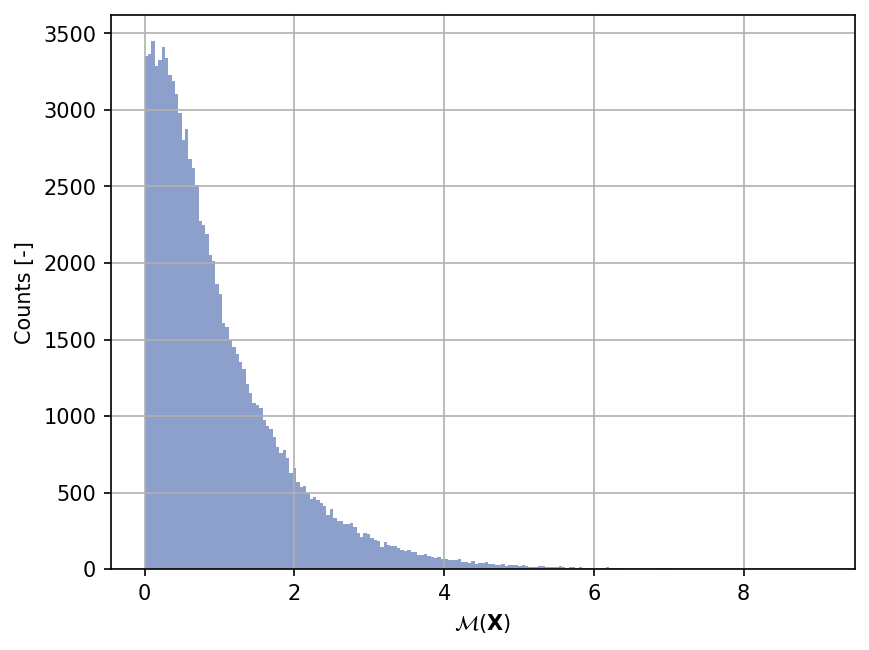
Sample histogram#
Shown below is the histogram of the output based on \(100'000\) random points:
Definite integration#
The integral value of the function over the whole domain \([0, 1]^M\) is analytical:
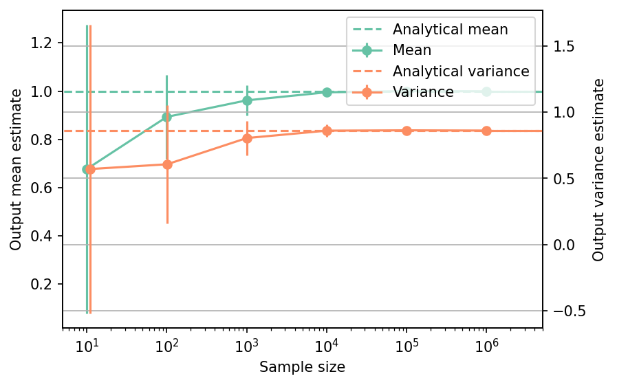
Moments estimation#
The mean and variance of the Sobol’-G function can be computed analytically,
and the results are:
\(\mathbb{E}[Y] = 1.0\)[3]
\(\mathbb{V}[Y] = \prod_{m = 1}^{M} \frac{\frac{4}{3} + 2 a_m + a_m^2}{(1 + a_m)^2} - 1\)
Notice that the value of the variance depends on the choice of the parameter values.
Shown below is the convergence of a direct Monte-Carlo estimation of the output mean and variance with increasing sample sizes compared with the analytical values. The error bars corresponds to twice the standard deviation of the estimates obtained from \(50\) replications.
The tabulated results for each sample size is shown below.
| Sample size | Mean | Mean error | Variance | Variance error | Remark |
|---|---|---|---|---|---|
| nan | 1.0000e+00 | 0.0000e+00 | 8.6088e-01 | 0.0000e+00 | Analytical |
| 1.0e+01 | 6.7700e-01 | 5.9851e-01 | 5.7055e-01 | 1.0925e+00 | Monte-Carlo |
| 1.0e+02 | 8.9314e-01 | 1.7460e-01 | 6.0670e-01 | 4.4630e-01 | Monte-Carlo |
| 1.0e+03 | 9.6174e-01 | 6.2156e-02 | 8.0497e-01 | 1.3128e-01 | Monte-Carlo |
| 1.0e+04 | 9.9519e-01 | 1.7246e-02 | 8.6095e-01 | 4.5081e-02 | Monte-Carlo |
| 1.0e+05 | 1.0000e+00 | 6.6156e-03 | 8.6369e-01 | 1.4632e-02 | Monte-Carlo |
| 1.0e+06 | 9.9927e-01 | 1.8470e-03 | 8.6172e-01 | 4.3970e-03 | Monte-Carlo |
References#
Andrea Saltelli and Ilya M. Sobol'. About the use of rank transformation in sensitivity analysis of model output. Reliability Engineering & System Safety, 50(3):225–239, 1995. doi:10.1016/0951-8320(95)00099-2.
Paul Bratley, Bennett L. Fox, and Harald Niederreiter. Implementation and tests of low-discrepancy sequences. ACM Transactions on Modeling and Computer Simulation, 2(3):195–213, 1992. doi:10.1145/146382.146385.
Xifu Sun, Barry Croke, Anthony Jakeman, and Stephen Roberts. Benchmarking Active Subspace methods of global sensitivity analysis against variance-based Sobol’ and Morris methods with established test functions. Environmental Modelling & Software, 149:105310, 2022. doi:10.1016/j.envsoft.2022.105310.
Amandine Marrel, Bertrand Iooss, Béatrice Laurent, and Olivier Roustant. Calculations of Sobol indices for the Gaussian process metamodel. Reliability Engineering & System Safety, 94(3):742–751, 2009. doi:10.1016/j.ress.2008.07.008.
Igor Radović, Ilya M. Sobol', and Robert F. Tichy. Quasi-Monte Carlo methods for numerical integration: comparison of different low discrepancy sequences. Monte Carlo Methods and Applications, 2(1):1–14, 1996. doi:10.1515/mcma.1996.2.1.1.
Ilya M. Sobol'. On quasi-Monte Carlo integrations. Mathematics and Computers in Simulation, 47(2-5):103–112, 1998. doi:10.1016/s0378-4754(98)00096-2.
Amandine Marrel, Bertrand Iooss, François Van Dorpe, and Elena Volkova. An efficient methodology for modeling complex computer codes with Gaussian processes. Computational Statistics & Data Analysis, 52(10):4731–4744, 2008. doi:10.1016/j.csda.2008.03.026.
Sergei Kucherenko, Balazs Feil, Nilay Shah, and Wolfgang Mauntz. The identification of model effective dimensions using global sensitivity analysis. Reliability Engineering & System Safety, 96(4):440–449, 2011. doi:10.1016/j.ress.2010.11.003.
Thierry Crestaux, Jean-Marc Martinez, Olivier Le Maître, and Olivier Lafitte. Polynomial chaos expansion for uncertainties quantification and sensitivity analysis. Presented at the Fifth International Conference on Sensitivity Analysis of Model Output, 2007. URL: http://samo2007.chem.elte.hu/lectures/Crestaux.pdf.